Key Takeaways
- High-fidelity CFD and real-time control can coexist through reduced-order modeling
- POD extracts dominant flow physics using linear algebra, no guessing required
- Reynolds number scaling verified the decomposition captures real fluid behavior
- Automated Python pipelines are essential for million-point datasets
The Problem
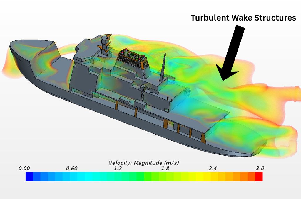
Landing a UAV on a moving ship is brutal. The superstructure creates turbulent wake, vortices, and unsteady pressure fields that destabilize the vehicle on final approach. Controllers need disturbance models, but ship-wake data is expensive and hard to get.
My research: generate high-fidelity CFD of ship wake flows, then compress them into models small enough for real-time control.
CFD Pipeline
Everything runs in OpenFOAM. Ship geometry imported as STL, fluid domain built and refined around it.
Solver: pimpleFoam with Large Eddy Simulation for unsteady turbulence. Mesh: ~2M hex-dominant cells, refined near hull and wake region. Numerics: Courant ≤ 0.5, adaptive timestep, parallelized across 13 cores.
Why Raw CFD Doesn't Work
The scale problem
Each run exports ~100 timesteps × 3 velocity components × 1M spatial points. That's 300 million numbers per simulation. Real-time control needs microsecond evaluations. The solution: extract the essential physics into a compact form.
POD: Proper Orthogonal Decomposition
POD decomposes flow fields into orthogonal spatial modes ranked by energy. The first few modes capture dominant physics; the rest can usually be dropped.
Where ū(x) is the mean flow, φk(x) are spatial modes, and ak(t) are temporal coefficients. Computed via SVD of the snapshot matrix. Typically, the first handful of modes capture >95% of flow energy, compressing down from millions of spatial vectors to dozens of coefficients.
Process: Stack velocity snapshots into matrix → subtract mean → SVD → keep top r modes → project onto reduced basis.
Verification
Key check: as wind speed (Reynolds number) increases, turbulence intensifies and more modes should be needed. I ran POD at multiple speeds and confirmed higher Re flows required more modes, matching the physics of turbulent energy distribution across scales.
Next Steps
- Check if temporal coefficients stay consistent across 4.5 to 5.5 m/s range for interpolation
- Literature review on stochastic noise injection for unresolved turbulence
- Ship motion correction (currently stationary in CFD domain)
- Explore Dynamic Mode Decomposition as POD alternative